
Home country bias is the one allocation decision most people have already made without ever making it. Nothing was chosen. The broker was local, the payroll was local, the index everyone quotes on the news was local, and the portfolio quietly ended up sitting almost entirely inside one country’s market and one currency.
The usual response to this is a vague instruction to “diversify internationally,” followed by an argument about how much, which nobody wins because it depends on an input nobody can pin down. That argument is the reason most portfolios never move at all.
This article skips the argument. The arithmetic that governs the decision is closed — it can be worked out on paper, from stated assumptions, with no forecast in it. And it produces a result that is genuinely surprising: the amount of the benefit depends heavily on the number you cannot pin down, but where the benefit sits on the curve barely depends on it at all.
Home country bias is a position you never chose
Start with the structural description, because the emotional one gets in the way. A portfolio concentrated in a single national market is a portfolio making one very large active bet: that the companies domiciled inside one set of borders will do at least as well as the companies outside them.
That may turn out to be right. It is still a bet, and it is a bet of a size almost nobody would place deliberately. If you were handed a blank sheet and asked what share of the world’s productive assets you wanted to own, the honest answer would rarely be “all of it from one country.”
The reason this passes unnoticed is that it does not feel like a position. It feels like the absence of one. The same illusion shows up with cash, which is why cash is a position, not the absence of one. Doing nothing is a choice with a payoff profile, and home country bias is the geographic version of that.
There is a second reason it survives. It is frequently rewarded. A concentrated position in a market that outperforms looks like conviction in hindsight, and the years where it works are the years that get remembered. That is the standard structure of an unmeasured risk: it pays until it does not, and the bill arrives in one piece.
The two risks you bundle by staying home
The phrase “investing internationally” hides the fact that it is two separate decisions, with different mechanics and different fixes. Treating them as one is the single most common error in this area.
The first is concentration. Your equity is exposed to one economy, one regulatory regime, one set of dominant sectors. Most national markets are far more sector-lopsided than their headline index count suggests, so this is usually a bigger bet than it looks.
The second is currency. Assets priced in another currency deliver a return in that currency, which you then convert. That conversion is a second, independent source of movement layered on top of the first.
These do not have to be accepted or rejected together. You can take the foreign equity exposure and neutralise most of the currency movement, or take both. That is a real choice with a computable answer, and it is covered further down.
It matters that they are separated, because they behave differently. Concentration is a risk you reduce by spreading. Currency is a risk that can partially cancel against the thing it is attached to — which, as we will see, sometimes makes the “safer” option the more volatile one.
What the variance arithmetic actually says
Here is the whole model. Split the equity portfolio into two blocks: a home block with weight w, and a rest-of-world block with weight 1 − w. Assume both blocks have the same volatility and a correlation of rho between them. The portfolio’s volatility, relative to holding the home block alone, is:
relative volatility = square root of [ w² + (1 − w)² + 2 × w × (1 − w) × rho ]
Three assumptions are doing work there and they should be named rather than buried. Both blocks are assumed to have equal volatility. No expected-return difference is assumed in either direction. And it is a single-period variance calculation, which is not the same thing as a lived experience over thirty years.
Those assumptions are deliberately neutral. The point of this calculation is not to predict which market wins. It is to isolate the one effect that does not require a forecast: what happens to the spread of outcomes when you stop holding one block and start holding two.
With equal volatilities, the minimum sits at w = 0.5 regardless of what rho is. That is worth pausing on. The location of the bottom of the curve does not depend on the correlation at all — only the depth of it does.
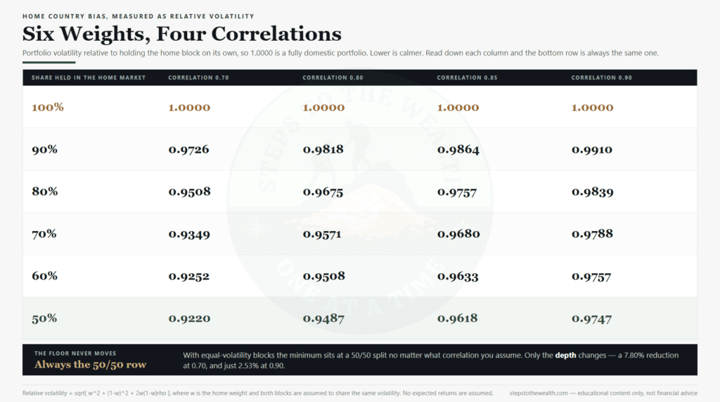
Read down any column and the same thing happens. The numbers fall fastest at the top and then flatten out. At a correlation of 0.85, the single move from 100% to 90% buys more than the entire journey from 70% down to 50%. The curve is steep where you start and nearly flat where the arguments happen.
The shape survives the assumption you cannot pin down
Now the part that makes this worth writing. The correlation between two large equity markets is the input everybody argues about, and reasonable people put it anywhere from 0.60 to 0.95 depending on the period and the pair.
That range changes the size of the prize enormously. At a correlation of 0.70, moving from fully home to a 50/50 split cuts volatility by 7.80%. At 0.90 the same move cuts it by only 2.53%, barely a third as much. If your question is “how much is this worth,” the answer genuinely does depend on a number nobody can hand you.
But that is not the question you have to answer. The question you have to answer is where to sit, and the shape of the curve is almost unmoved:
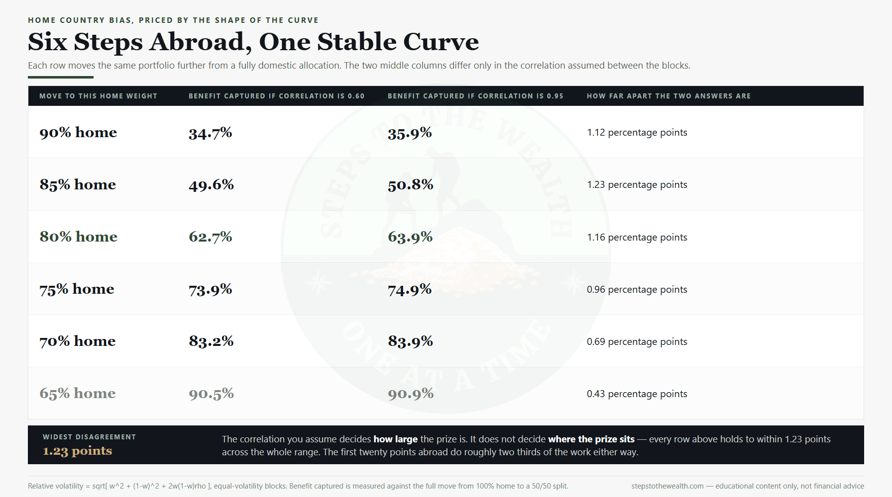
Across correlations from 0.60 to 0.95, the share of the total available reduction captured by moving the first twenty points abroad runs 62.7%, 63.1%, 63.4%, 63.5%, 63.7%, 63.9%. That is a spread of 1.16 percentage points across the entire plausible range of the input.
The halfway mark is just as stable. Moving only fifteen points abroad — to 85% home — captures right about 50% of everything on offer, varying from 49.6% to 50.8% across the same range.
This is the practical result, and it is the opposite of what the usual debate implies. You do not need to resolve the correlation argument to act. The correlation argument determines how much you gain. It does not meaningfully determine where the gains are, and the gains are overwhelmingly at the start.
That is a familiar shape if you have read how diversification reduces risk: the first few steps away from concentration do most of the work, and the returns to further spreading fall away fast. What is new here is that the shape is measurably insensitive to the assumption, which is what lets you act without winning the argument first.
Where the decision actually lives
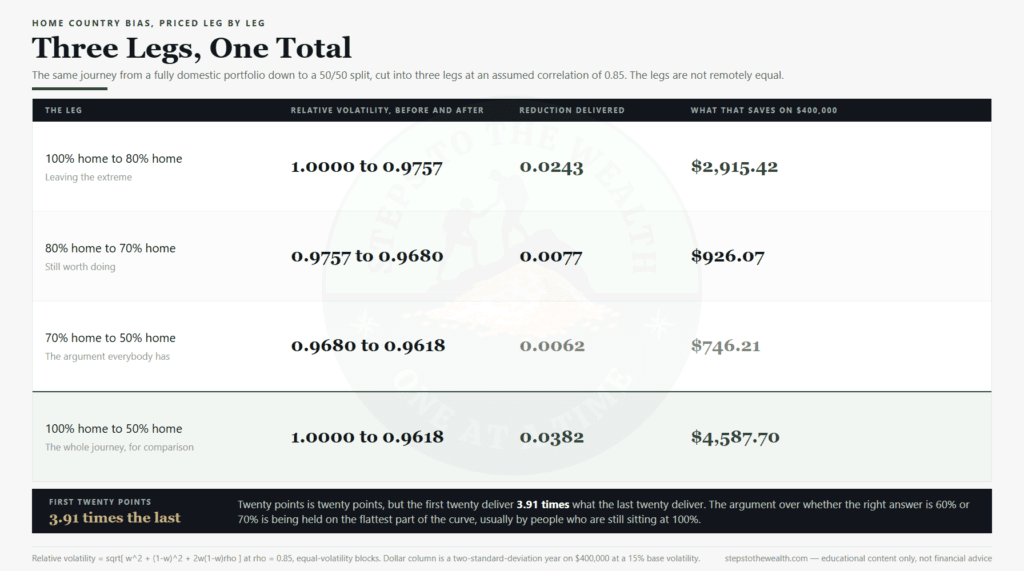
Take a correlation of 0.85, roughly the middle of the plausible range, and price three moves against each other.
Going from 100% home to 80% home drops relative volatility from 1.0000 to 0.9757, a fall of 0.0243. Going from 80% to 70% drops it to 0.9680, a further 0.0077. Going all the way from 70% to a 50/50 split drops it to 0.9618, a further 0.0062.
So the first twenty points are worth 3.91 times as much as the last twenty. Every hour spent debating whether the right answer is 60% or 70% is being spent on the flattest part of the curve, by people who are usually still sitting at 100%.
This is a calibration point rather than a recommendation. It says the cost of being approximately right is small and the cost of being at the extreme is large. It does not say what your number should be, because that depends on things this arithmetic does not contain.
It also reframes what a mistake looks like. Landing at 75% when 65% was marginally better is a rounding error. Sitting at 100% because the debate was unresolved is the entire effect.
What the reduction is actually worth in money
Percentages of volatility are easy to nod along to and hard to feel, so price it.
Take a $400,000 equity portfolio and assume 15% annual volatility for a fully home allocation. A two-standard-deviation year — the kind that happens, not the kind that is unthinkable — is a 30.00% move, or $120,000.
Move to 80% home at a correlation of 0.85 and volatility falls to 14.6356%. The same two-sigma year is now 29.2711%, or $117,084.58. You have saved $2,915.42 on a $400,000 portfolio.
Go all the way to 65% home and the saving reaches $4,167.36. That is the whole prize, and it is worth stating plainly rather than dressing it up: as a volatility trade, spreading out geographically is a modest improvement, not a transformation.
If that were the entire case, it would be reasonable to ignore it. It is not the entire case, and the more important half does not show up in a variance calculation at all.
Volatility understates the argument
A variance model treats a bad outcome as a wide distribution around a fixed centre. It assumes the centre is in the right place. The risk that actually justifies geographic spreading is the risk that the centre itself is wrong for a very long time.
A single national market can trail the rest of the world for a decade or more without ever crashing, because its dominant sectors mature, its demographics turn, or its currency erodes against the things its holders want to buy. None of that registers as volatility. It registers as a portfolio that is calm and going nowhere.
That is the asymmetry worth acting on. The volatility saving is small and reliable and computable. The protection against a long, quiet, structural underperformance is large and not computable, which is precisely why it gets left out of the argument, and why the argument stays stuck on the smaller half.
Hedging is a second decision, with its own threshold
Now the currency half, which has a cleaner answer than its reputation suggests.
Holding foreign equity without hedging means your return in home-currency terms is roughly the asset’s return plus the currency’s move. The volatility of that combination is not simply the sum of the two. It is:
unhedged variance = sigma_e² + sigma_c² + 2 × rho × sigma_e × sigma_c
where sigma_e is the equity volatility, sigma_c the currency volatility, and rho the correlation between them. Hedging removes the currency terms and leaves sigma_e².
Set the unhedged variance below the hedged variance and almost everything cancels. What survives is a single condition:
unhedged is less volatile than hedged when rho is below −½ × (sigma_c ÷ sigma_e)
The threshold depends only on the ratio of the two volatilities. With equity volatility at 15% and currency volatility at 8%, the crossing point is a correlation of −0.2667. Above that, hedging lowers volatility. Below it, hedging raises volatility, because you have removed something that was partially offsetting your equity moves.
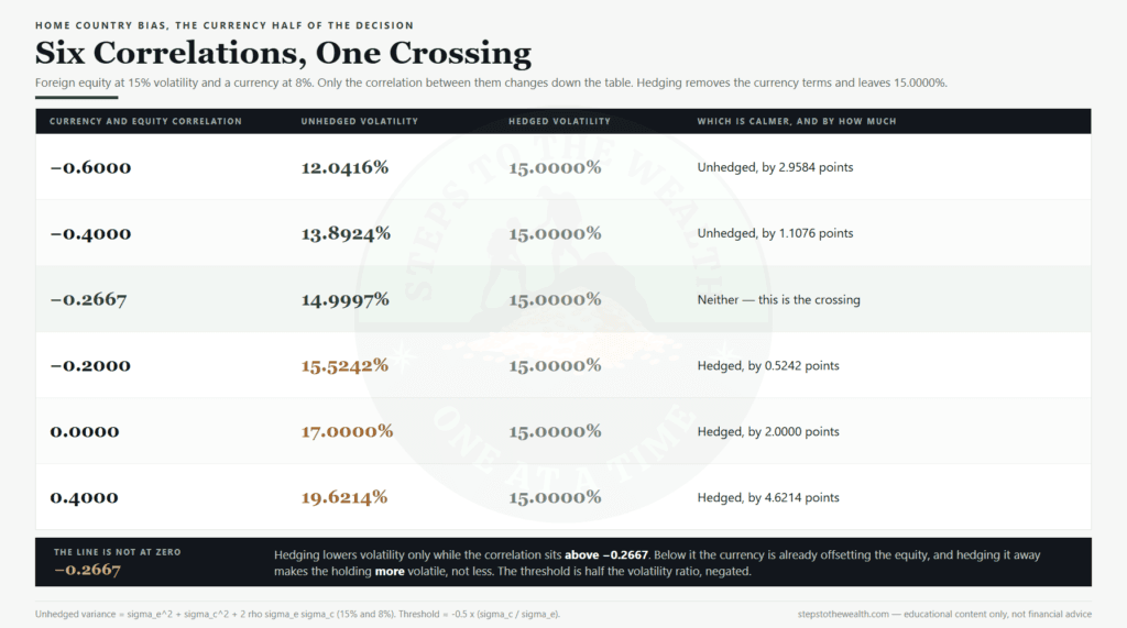
The number that matters is that the threshold is not zero. The intuitive rule — hedge unless the currency moves with your equities — puts the line in the wrong place. A currency can be mildly negatively correlated with foreign equity and hedging it still reduces your volatility.
Work the same numbers the other way and the magnitudes appear. At a correlation of zero, unhedged volatility is 17.00% against 15.00% hedged. At −0.40 it is 13.89% against 15.00%, so the unhedged holding is the calmer one. At +0.40 it is 19.62%, and the currency is amplifying rather than offsetting.
None of this prices the cost of hedging itself, which is real and which pushes the practical threshold further in favour of leaving it alone. It also says nothing about long horizons, where currency effects behave differently from a single-period variance calculation. It is a floor for thinking, not a rule to apply blind.
What this arithmetic will not tell you
Every model earns its keep by being explicit about what it excludes, so here is the list.
It assumes equal volatility in both blocks. If your home market is materially more or less volatile than the rest of the world, the minimum moves away from 50/50. The direction is intuitive — the calmer block gets more weight — but the exact point changes.
It contains no expected returns. This is a pure risk calculation. It does not claim that spreading out earns you more. It claims it makes the spread of outcomes narrower, which is a different and more defensible claim.
It is single-period. Volatility over one period is not the same as the risk of a bad sequence arriving at the wrong moment. That is a separate problem, and if your money has a date on it the relevant analysis is in investing for short-term goals.
It ignores costs, taxes and access. Foreign exposure can carry higher fees, withholding complications and platform limitations. Those are real and they are jurisdiction-specific, which is exactly why this article does not name any jurisdiction. The arithmetic is universal. The friction is not.
Correlations are not stable. They rise in crises, which is when diversification is most wanted and least delivered. That failure mode is documented in the portfolio stress test, and it is the strongest honest argument against expecting too much from any of this.
Taken together those caveats do not overturn the result. They bound it. The first steps abroad still do most of the work, and the shape is still robust to the input you cannot pin down. The caveats say the effect is smaller and messier than the clean numbers imply, not that it runs the other way.
How to measure your own home country bias this week
This takes about twenty minutes and needs no tooling beyond a spreadsheet.
First, list every equity holding with its value, and mark each one by the market it is actually exposed to rather than where you bought it. A locally listed fund tracking a global index is not home exposure. A locally listed company earning most of its revenue abroad is a genuinely ambiguous case — note it and move on.
Second, add up the home-exposed share as a percentage. That single number is your w. Most people who have never run this are surprised by how close to 100 it is.
Third, do the same for currency. Which share of the portfolio ultimately pays out in your spending currency, and which does not? This will not match the first number, and the gap between them is the thing most portfolios have never looked at.
Fourth, check whether your largest single exposure is a decision or an accident. If your employer’s equity is in there too, the concentration is worse than the geography suggests, and equity compensation risk covers that interaction directly.
Fifth, decide once and write the target down with a rebalancing rule attached. A number you have committed to in advance is worth more than a better number you renegotiate every quarter, which is the whole argument for rules-based investing.
For a broader framing of how allocation decisions fit together, the regulator-published primer on asset allocation is a reasonable neutral starting point.
Frequently asked questions
Is home country bias always a mistake? No. It is always a position, which is a different claim. There are defensible reasons to hold more of your home market than its global weight, including that your liabilities are denominated in your own currency. What is not defensible is holding it at 100% because nobody ever measured it.
What is the right percentage? This arithmetic does not produce one, and anyone who gives you a single universal number is not reading the same curve. What it produces is a ranking of where effort is worth spending: the move away from the extreme matters, the fine-tuning does not.
Does this mean I should hedge my currency exposure? It means the question has a threshold rather than a default. Above a correlation of about −0.27, on the volatilities used here, hedging reduces volatility. Below it, hedging adds volatility. Hedging costs then push the practical answer further toward leaving it unhedged.
Does volatility even matter if I am investing for decades? Less than most people assume, and that is the honest answer. Volatility is not the same thing as risk, a distinction worked through in volatility is not risk. The concentration argument survives that objection better than the volatility argument does, because a single-country bet can be permanently wrong rather than merely bumpy.
What if my home market has outperformed for years? Then your home country bias has been paying, and you have no way to know from that fact alone whether it was skill in the selection or luck in the period. Past outperformance is the weakest available evidence for future concentration.
The number is the point, not the argument
The debate about international allocation is stuck because it is being conducted about the wrong quantity. People argue about correlation, which determines the size of the prize, and then treat the unresolved argument as a reason to stay at the extreme.
The curve does not care. Across every plausible correlation, the first twenty points abroad deliver about 63% of everything available, the first fifteen deliver about half, and the last fifteen deliver almost nothing. That is a calibration you can act on without predicting anything.
Measure your w this week. If it starts with a 9, the arithmetic has something to say to you. If it is already in the sixties or seventies, the remaining decision is a rounding error and your attention belongs somewhere else.
If you want the framework pieces as they are published, they go out through the newsletter.
Educational content only — not financial advice. The calculations here are illustrative, derived from stated assumptions, and are not a forecast or a recommendation. Costs, taxes and access rules vary by the jurisdiction in which you reside.