
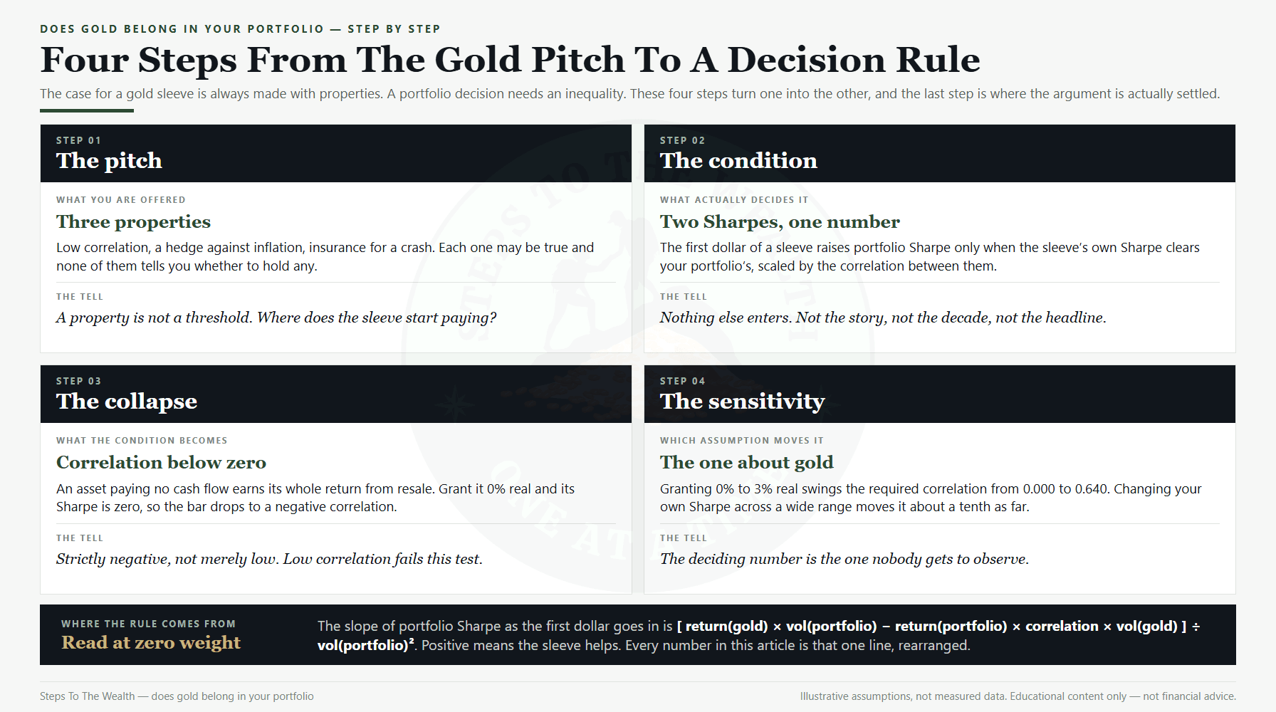
Ask whether a gold sleeve belongs in a portfolio and you get properties back. It hedges inflation. It has low correlation with equities. It is insurance for a crash. Each of those may be true. None of them is a decision rule, because a property describes what an asset is like — not what it does to the thing you already own.
Does gold belong in your portfolio is a marginal question, not a standalone one. You are not asking whether gold is a good asset in the abstract. You are asking whether moving the first dollar out of what you hold and into gold makes the whole book better on a risk-adjusted basis. That question has an exact answer. It is one inequality long, and almost nobody states it.
What follows is that inequality, where it comes from, what it collapses to when the asset pays you nothing while you hold it, and how much the answer is actually worth if it comes out in gold’s favour. Every number here is closed from assumptions stated on the page. Nothing is sourced from a backtest, because the input that decides this is not one you can measure.
Does gold belong in your portfolio, or does gold just go up?
Those are different questions and the second one is easier, which is why it gets answered instead. An asset can rise for a decade and still be a bad addition. An asset can lag badly and still be a good one. What matters at the margin is not the return by itself but the return relative to the volatility it brings, and how that volatility interacts with the volatility you already carry.
The standard measure of that trade is the Sharpe ratio: excess return divided by volatility. If the phrase is new, the mechanics and the three ways the number misleads are covered in how the Sharpe ratio actually works. For this article you only need the shape of it. Higher is better. Two assets can be compared by it. And critically, a portfolio has one of its own.
So the real question is narrow. Does the portfolio’s Sharpe ratio go up when the first dollar of gold goes in? Not the tenth percent. The first dollar. If the first dollar does not help, no amount of it helps, and the sizing conversation never needs to happen.
The condition that decides whether any sleeve earns its place
Write the portfolio as your existing book plus a small weight in the new sleeve. Take the slope of the portfolio’s Sharpe ratio as that weight moves off zero. The algebra is short and the result is clean:
The slope at zero weight is [ return(gold) × vol(portfolio) − return(portfolio) × correlation × vol(gold) ] ÷ vol(portfolio)²
Set that above zero and divide through. Everything cancels except a comparison between two Sharpe ratios and the correlation between the two holdings:
Gold’s Sharpe ratio must exceed the correlation multiplied by your portfolio’s Sharpe ratio.
That is the whole test. Two Sharpe ratios and one correlation. Not the price of the metal, not the decade it had, not the geopolitical story attached to it. Those things matter only insofar as they change one of the three numbers, and if they do not change one of the three numbers, they do not change the answer.
Read what the condition is doing. Correlation is the discount. When the sleeve moves independently of what you own, the bar it must clear drops. When it moves with what you own, the bar rises toward your own Sharpe ratio, which is a high bar for anything to clear. At a correlation of 1.00 the sleeve has to beat your portfolio outright, which is just the statement that a perfect substitute has to be better to be worth swapping into.
Notice what is not in the condition: any notion of the sleeve being safe, familiar, tangible, or a store of value. Those are descriptions. They enter the arithmetic only through return, volatility and correlation, or they do not enter at all.
Why an asset with no cash flow collapses the condition
Here is where gold separates itself from the rest of the allocation debate. A share of a business has an internal return engine. It produces profit, and some of that profit reaches you as dividends or as retained earnings that compound inside the company. A bond pays a coupon. Rental property pays rent. Whatever you think those cash flows are worth, they exist, and they are what you actually own when you buy the asset.
Gold produces nothing. It sits. Its entire real return, over any period you care about, is the difference between what you paid and what somebody else is willing to pay later. That is not a criticism of the metal. It is a description of the return mechanism, and it has a direct consequence for the test above.
If you decline to forecast what a future buyer will pay — if you grant gold zero percent real return over the long run, on the grounds that you have no mechanism to point at — then gold’s Sharpe ratio is zero. Put zero on the left side of the condition and it collapses to something stark:
The correlation must be strictly below zero.
Not low. Not near zero. Negative. Under a zero-return grant, a sleeve that is merely uncorrelated does nothing for the portfolio’s Sharpe ratio, and a sleeve that is even slightly positively correlated makes it worse. The most common sentence in the pro-gold case, that it has low correlation with equities, fails this version of the test outright.
Of course you may not want to grant zero. Grant more and the bar rises with it. The table below runs the ladder, holding the equity side at a 5% real excess return with 16% volatility — a Sharpe ratio of 0.3125 — and gold at 15% volatility throughout.
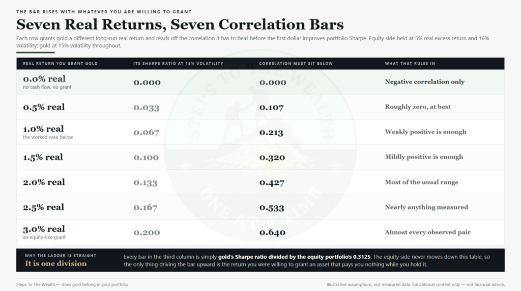
The ladder is a straight line because it is one division. Every bar in the third column is gold’s Sharpe ratio divided by 0.3125. Grant half a percent real and you need a correlation under 0.107, which is still effectively an uncorrelated-or-better requirement. Grant a full percent and the bar reaches 0.213. Grant three percent, close to what people assume for equities after inflation, and almost any correlation ever measured would qualify.
So the answer to the question is not fixed. It swings on the grant. Which raises the obvious follow-up: how confident should anyone be about that number?
The assumption that decides it is the one you cannot observe
Every model has inputs, and the useful question is never whether the inputs are uncertain. They always are. The useful question is which input the answer is actually resting on. Vary each one across a plausible range and see which one moves the conclusion.
Do that here and the result is uncomfortable. Vary your own equity Sharpe ratio from 0.25 to 0.40 — a range far wider than anyone seriously argues about — and the correlation bar moves from 0.267 to 0.167. A swing of 0.100. Now vary the grant on gold from 0% to 3% real and the same bar moves from 0.000 to 0.640. A swing of 0.640.
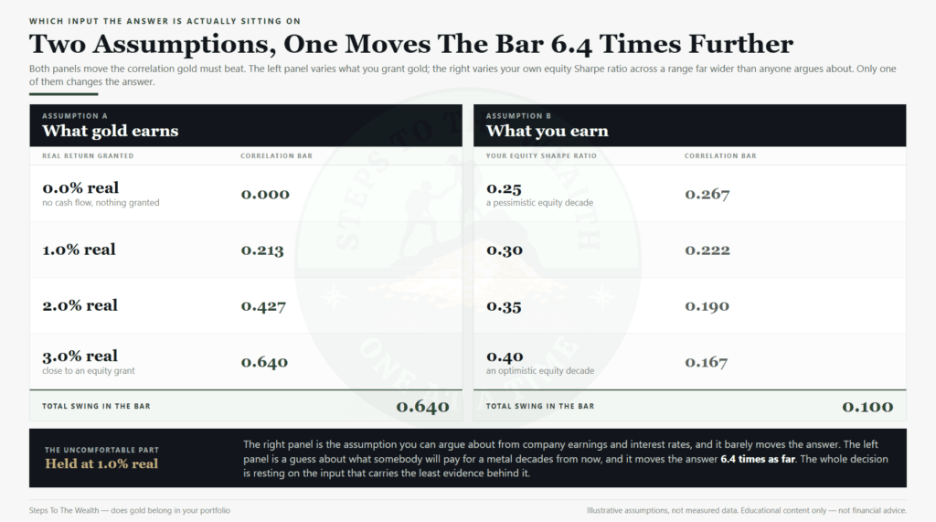
The assumption about gold moves the answer 6.4 times as far as the assumption about your own portfolio. That ratio is the argument, and it is worth sitting with for a moment, because of what the two assumptions are made of.
Your equity Sharpe ratio is a guess, but it is a guess anchored to something. Companies report earnings. Yields are quoted. Valuations can be measured and argued about. You can be wrong about it, and people frequently are, but there is a mechanism underneath the number that you can reason from.
The grant on gold has no such anchor. There are no earnings to discount and no yield to quote. The number is a forecast of what a stranger will pay for a metal in twenty years, expressed as a compound rate. It is the softest input in the model, and it is the one carrying the decision.
This is not an argument that gold returns zero. It is an argument that the honest range on that input is wide, and that a wide range on the deciding input means the conclusion is not really being derived. It is being chosen and then dressed in arithmetic.
Suppose you are right. How big is the prize?
Grant the pro-gold case its best plausible footing and price it. If the condition passes, mean-variance optimisation will hand back a specific weight rather than a vague “five to ten percent”, and it will also tell you exactly what the improvement is worth.
Four cases, plus the two that produce nothing, on the same assumptions as before: equity at 5.00% real excess return and 16.00% volatility, gold at 15.00% volatility, long positions only.
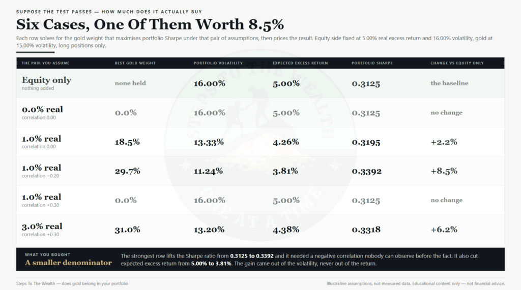
Read the strongest row first. Granting 1.0% real and a correlation of −0.20 — genuinely negative, which is a strong assumption — produces an optimal gold weight of 29.7% and lifts the portfolio Sharpe ratio from 0.3125 to 0.3392. That is the best outcome on the table, and it is an improvement of 8.5%.
Now read what it cost. Expected excess return falls from 5.00% to 3.81%. Volatility falls from 16.00% to 11.24%. The Sharpe ratio improved because the denominator shrank faster than the numerator, not because the portfolio earns more. You did not buy return. You bought a smaller denominator, and you paid 1.19 points of expected excess return for it.
The middle case is more sobering. At 1.0% real and zero correlation the optimiser wants 18.5% in gold and delivers a Sharpe ratio of 0.3195 — a 2.2% improvement, in exchange for cutting expected excess return by nearly three quarters of a point. That is a real gain. It is also small enough that a modest error in any of the three inputs erases it entirely.
And at 1.0% real with a correlation of +0.30, the optimiser wants a negative weight of about −11%. For anyone who is not shorting the metal, that means zero. The condition failed, and the honest allocation is none.
What the inflation hedge argument is actually claiming
The inflation case deserves separating out, because it sounds like it sits outside this framework and it does not.
Every return in this article is a real return — after inflation. That is deliberate, and it is the same discipline applied in the difference between a nominal and a real return. So the claim “gold protects you from inflation” is already inside the model. Translated, it is the claim that gold’s real return is at least zero across inflationary regimes, which is exactly the grant on the left side of the condition.
That reframing is useful because it makes the claim testable in principle and demanding in practice. A hedge that merely keeps pace with inflation delivers a 0% real return, which puts you back on the first row of the ladder, where nothing but a negative correlation gets the sleeve into the book. To beat that row, gold has to do more than track inflation. It has to compound above it.
There is a separate and more defensible version of the argument: that gold is not there to raise the Sharpe ratio at all, but to pay off in a specific regime where other things fail. That is a real position, and it is worth holding honestly. It is just not the same claim, and the arithmetic above cannot price it.
This is not the same question as home country bias
The variance arithmetic here looks similar to the arithmetic in the case for holding assets outside your own country, and the two arrive at opposite conclusions. The difference is worth naming, because conflating them is easy.
The geographic question splits one asset class across regions. Both legs are equities. Both legs have an internal return engine and a defensible positive expected return, so the grant that decides this article is not in dispute there. All that is being traded is correlation, and the answer comes out strongly in favour of diversifying, with the size of the prize varying but the direction holding across every correlation assumption tested.
Here, the direction itself flips depending on an unobservable input. That is the whole difference. In the geographic case the uncertain input changes how much you gain; in the gold case it changes whether you gain at all. Same family of algebra, different question, and a much weaker claim available at the end of it.
The broader holdings-level version of the argument — more positions, less single-name risk — is covered separately in how diversification actually reduces risk, and none of it depends on the grant either.
What this test does not cover
Four honest limits, because a framework that only ever supports one conclusion is not a framework.
It is a two-moment test. Return and volatility, nothing else. It has no view on skew, on fat tails, or on what happens in the worst week of a decade. If your reason for holding gold is a specific crash scenario rather than a smoother ride, this test is answering a question you did not ask. Volatility and risk are not the same thing, and the Sharpe ratio only knows about the first one.
Correlation is not a constant. The single number in the condition is an average over whatever window you measured, and correlations between asset classes drift, sometimes sharply, exactly when it matters. A sleeve that qualified on a twenty-year average can fail badly in the eighteen months you needed it. Running a book through several regimes rather than one, as in stress-testing a portfolio across history, shows how far a gold sleeve’s behaviour moves between decades.
It ignores costs. Fund fees, spreads, storage and, depending on where you live, a different tax treatment for metals than for equities. All of those come out of the grant. A sleeve granted 1% real and charged 0.4% in fees is really being granted 0.6%, and on the ladder that moves the required correlation from 0.213 down to 0.128.
It says nothing about rebalancing. A volatile, weakly correlated sleeve held at a fixed target weight generates its own rebalancing flow, which is a separate source of return and a separate discipline problem. That is its own subject, handled in rebalancing versus chasing.
Running the numbers that are actually yours
Everything above uses one illustrative equity portfolio. Yours is different, and the condition is sensitive to the numbers you put in it, so the useful move is to run it rather than read it.
Three inputs, in order of how much they matter. First, the real return you are genuinely willing to grant gold, written down before you look at anything else, because writing it down afterwards is just reverse-engineering. Second, the correlation you are assuming, and over which window. Third, your own portfolio’s Sharpe ratio, which is the input that matters least and gets debated most.
Then run the division. Gold’s Sharpe ratio is your grant divided by its volatility. The bar is that number divided by your portfolio’s Sharpe ratio. If your assumed correlation sits below the bar, the sleeve earns a place and the optimiser will size it. If it does not, the honest answer is zero, and zero is a position — the same way holding cash is a position rather than an absence of one.
If you would rather see the behaviour than the algebra, gold and the rest of the metals sit in the commodity list inside the DCA Simulator, alongside equities and crypto, so you can run the same contribution plan into a gold sleeve and into an index and compare what each one actually did over the window you choose. Historical behaviour is not the grant, and it should not be mistaken for it, but it does put a range around what you are assuming. For a wider view of how allocation decisions are usually framed, the SEC’s investor education material on asset allocation is a plain-language starting point.
The operator’s version
Strip it down to what you would actually run.
A sleeve improves your portfolio’s risk-adjusted return only when its own Sharpe ratio clears your portfolio’s, scaled down by the correlation between them. That is the entire test, and it applies to every candidate asset, not only this one.
For an asset that pays no cash flow, the left side of that test is a forecast of resale price and nothing else. Grant it zero and the condition demands a strictly negative correlation, which is a much harder requirement than the low correlation usually offered. Grant it more and the bar rises with the grant, in a straight line.
The deciding assumption is the one about the asset, not the one about you — it moves the answer 6.4 times as far — and it is the one with the least evidence behind it. When the answer to does gold belong in your portfolio depends almost entirely on the softest number in the model, the correct posture is not confidence in either direction. It is a small position held with stated assumptions, or no position held for a stated reason. Both are defensible. What is not defensible is a number chosen because it felt prudent and then justified with properties.
And if the test does pass on your numbers, size it with the optimiser rather than with a round figure, and remember what you bought. In the strongest case on this page the improvement was 0.0267 of a Sharpe ratio, purchased with 1.19 points of expected excess return. That is what a good outcome looks like here. It is worth having. It is not worth arguing about for a decade.
If you want the weekly version of this — risk readings on five major assets and what the framework says to do about them — that is what the Sunday newsletter is for.
Educational content only — not financial advice. Every figure on this page is closed from the assumptions stated beside it and is illustrative, not a measurement or a forecast.