
A dynamic DCA strategy is dollar-cost averaging with one thing added: the size of each buy is set by a risk reading rather than being the same every month. Everything else is unchanged. Same assets, same automation, same schedule, same long horizon. One column of a table does all the work.
That is a smaller idea than the name suggests, and the smallness is the point. Static dollar-cost averaging deliberately ignores price so that you cannot talk yourself out of buying. It works, and it works mostly because it removes you from the decision. The cost of that design is that it also ignores the one piece of information you actually have: whether the thing you are buying is currently cheap or currently stretched.
Dynamic DCA adds that information back without handing the decision to your judgement. The reading changes the size. The table decides what the size is. You execute.
Educational content only. Not financial advice.
What a dynamic DCA strategy actually is
Take an ordinary monthly contribution — call it $1,000 — and stop treating it as a fixed instruction. Instead, treat it as a base that gets multiplied by whatever the current risk reading says.
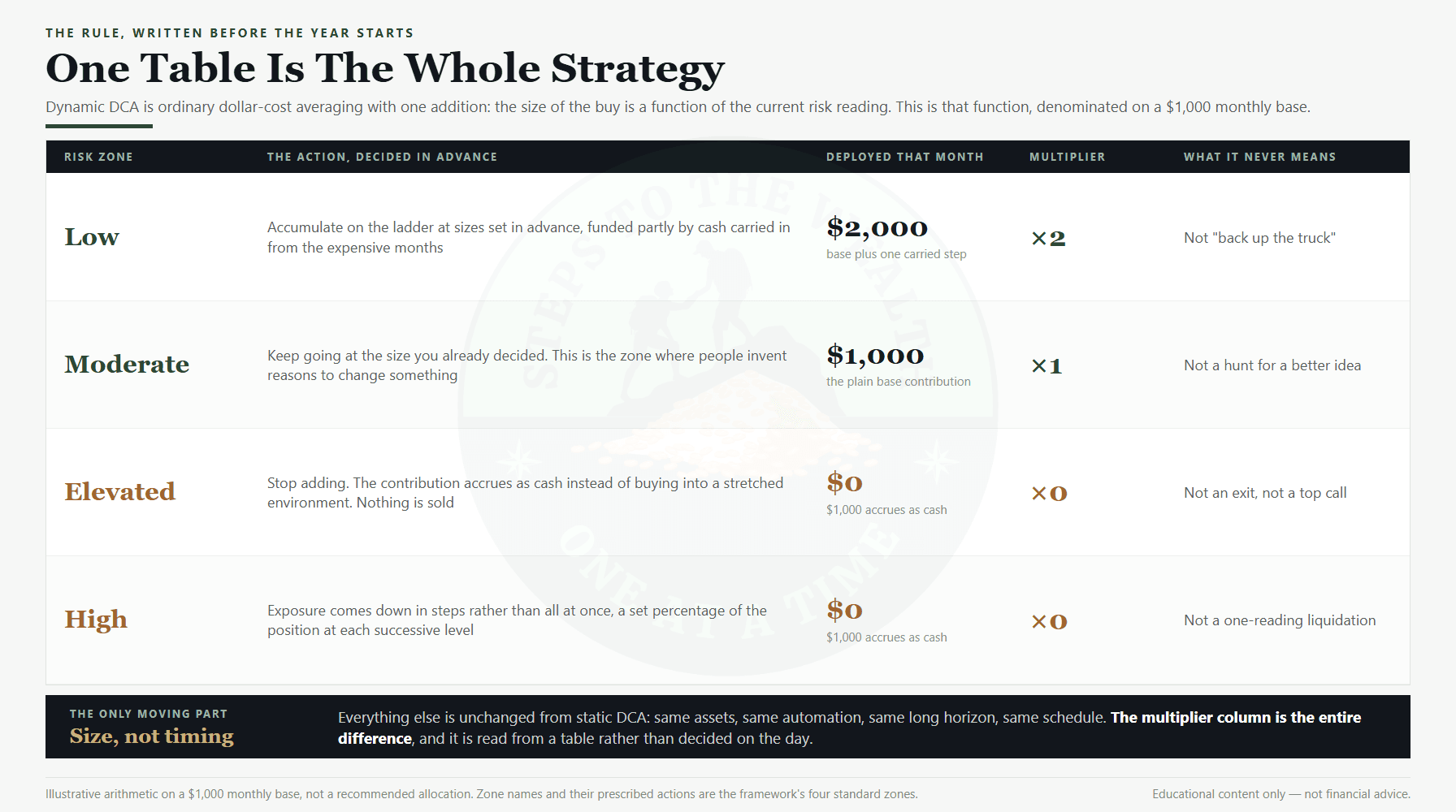
When risk reads low, the buy is larger than the base. When risk reads moderate, it is exactly the base. When risk reads elevated or high, nothing is bought at all, and the contribution accrues as cash instead. Four states, four sizes, and the mapping between them written down while you are calm and nothing is at stake.
What makes it a strategy rather than a mood is that the mapping exists before the reading arrives. You are not deciding on the day whether things feel expensive. You are looking up a level in a table you wrote months earlier, and executing the row it lands on.
This sits on top of a risk-first framework rather than replacing it. The framework’s job is to produce a reading that means something. Dynamic DCA’s job is to convert that reading into a dollar amount. Neither half is useful without the other: a reading with no prescribed action is trivia, and a prescribed action with no reading is a guess.
The four zones, and the one number that changes
The zones are the same four the framework always uses, and each one commits you to a single action.
Low. Accumulate on the ladder at sizes set in advance. On a $1,000 base that is $2,000 in the month — the base plus one step of the cash carried in from the expensive months. It is not “back up the truck”, because the size was fixed before the fall arrived and does not respond to how dramatic the fall feels.
Moderate. Keep going at the size you already decided. $1,000, unchanged. This is the zone where people invent reasons to change something, and the discipline being tested is the discipline of not improvising.
Elevated. Stop adding. The contribution accrues as cash rather than buying into a stretched environment. Nothing is sold, and this is not a forecast that a top is coming — it is a statement that the price you would be paying is poor relative to its own range.
High. Exposure comes down in steps, a set percentage of the position at each successive level, rather than all at once on a single reading. A staged exit that turns out to be early costs you a little. An all-at-once exit that turns out to be wrong costs you the recovery.
Notice what does not change across those four rows. Not the asset. Not the schedule. Not the automation. Not the horizon. The multiplier column is the entire difference between a dynamic DCA strategy and a static one, which is why the whole thing fits on a single table.
Same $12,000, different months
Here is the part that gets misunderstood most often. Dynamic DCA does not mean investing more money. It means investing the same money in different months.
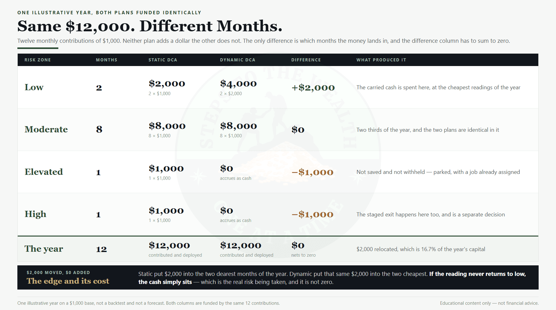
Take one illustrative year: twelve contributions of $1,000, so $12,000 in total. Suppose the readings across that year land as two low months, eight moderate, one elevated and one high.
The static plan deploys $1,000 twelve times: $12,000, evenly spread. The dynamic plan deploys $2,000 in each of the two low months, $1,000 in each of the eight moderate months, and nothing in the elevated and high months, where the $2,000 of contributions accrues as cash instead. That is $4,000 plus $8,000 plus zero plus zero, which is also $12,000.
Identical funding. Identical total deployed. The only difference is that $2,000 moved out of the two most expensive months of the year and into the two cheapest — 16.7% of the year’s capital, relocated. The cash that funded the extra buying is precisely the cash the elevated and high months refused to spend, which is why the two columns balance to the dollar.
This is also the honest answer to the lump sum versus dollar-cost averaging question. A risk-driven schedule is not chosen because it produces the highest expected return in a model. It is chosen because it is a schedule you will actually execute, and because it puts a larger share of the same money into the cheaper end of the range.
And it carries a real cost, which the arithmetic makes visible rather than hiding. If the reading never returns to low, the cash simply sits. It does not compound while it waits, and the price of waiting is not zero — that is exactly what waiting actually costs. Any version of this strategy that does not admit that is selling something.
Why a dynamic DCA strategy is not market timing
The objection arrives immediately and it deserves a real answer: if you are buying more sometimes and less other times, how is that not market timing with extra steps?
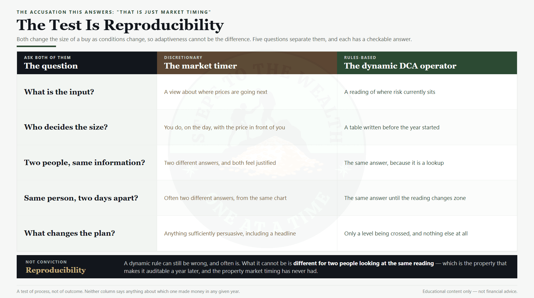
It cannot be that one adapts and the other does not, because both change the size of a buy as conditions change. The difference is where the decision lives.
A market timer’s input is a view about where prices are going next. The size is decided on the day, with the price on the screen. Two timers with the same information produce two different answers, and both feel justified. The same timer on two different days will often produce two different answers from the same chart. Anything sufficiently persuasive can change the plan, including a headline.
A dynamic DCA operator’s input is a reading of where risk currently sits. The size was decided in a table written before the year started. Two operators with the same reading produce the same answer, because it is a lookup rather than a judgement. The same operator produces the same answer until the reading crosses into a different zone. Only a level being crossed changes anything at all.
So the test is not conviction, and it is certainly not accuracy. A dynamic rule can be wrong, and frequently is: some elevated readings resolve upward, and some low readings are followed by another fall. What it cannot be is different for two people looking at the same number. That property is what makes the year auditable afterwards, and it is the property discretionary timing has never had. The distinction matters enough that most of the myths about dollar-cost averaging collapse once you separate “adapting by rule” from “predicting by feel”.
The other half: what the rule does on the way up
Most people meet dynamic DCA as an accumulation idea and stop there. The exit half is what makes it symmetric, and it is the half that is easier to skip.
At elevated readings, new money stops buying and accrues instead. Nothing is sold. This alone changes the shape of a portfolio over a cycle, because it stops you from adding at the worst prices without requiring you to predict anything.
At high readings, the position itself comes down in steps — a set percentage at each successive level, decided in advance. You will sell some of the position before the peak and some after it, and neither of those outcomes is a failure. Top-ticking is not on the menu, and a strategy that requires it is not a strategy.
Whether the exit half applies to you at all is a separate question about position size and horizon. If the position is small relative to your net worth and your horizon is genuinely multi-decade, holding through the drawdown is a defensible default. If the position has grown large relative to everything else you own, a staged reduction rule is the difference between a plan and a hope. That is a structural question about the portfolio rather than a question about the market, and it belongs in the annual review rather than in a weekly reading.
Where the edge actually comes from, and where it does not
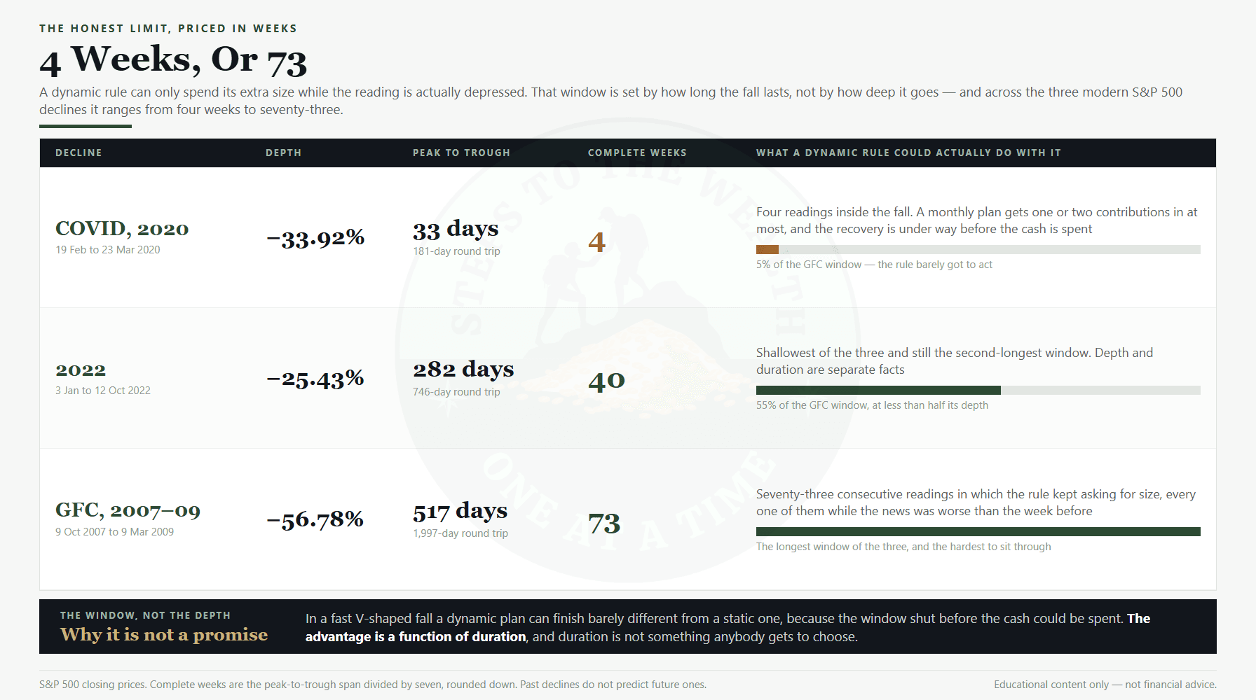
A dynamic rule can only spend its extra size while the reading is actually depressed. So the size of the advantage depends on how long the fall lasts, not on how deep it goes — and those two things are much less correlated than people assume.
Three modern S&P 500 declines make the point, measured on closing prices. The COVID fall of 2020 ran from 19 February to 23 March: 33.92%, in 33 days, which is four complete weeks. The 2022 decline ran from 3 January to 12 October: 25.43%, over 282 days, or 40 complete weeks. The financial crisis ran from 9 October 2007 to 9 March 2009: 56.78%, over 517 days, which is 73 complete weeks.
The shallowest of the three produced the second-longest window. The fastest produced almost no window at all. Four weekly readings is one or two monthly contributions at most, and the recovery was already under way before much cash could be spent — which is why a dynamic plan through the COVID crash can finish barely different from a static one.
The financial crisis is the opposite case, and not a comfortable one. Seventy-three consecutive readings in which the rule kept asking for size, every one of them arriving while the news was worse than the week before. That is what steady buying through 2008 actually required, and the difficulty was never the arithmetic. A volatile asset compresses the same lesson into a shorter and sharper window, which is what the 2021 to 2022 bitcoin drawdown shows.
The practical consequence is that a dynamic DCA strategy should be adopted for its structure, not for an expected outperformance number. In a fast V-shaped fall it can finish level with static DCA. In a long grind it has many more chances to deploy the carried cash. Nobody gets to choose which kind of decline they receive, so the honest framing is that the rule improves the distribution of what you pay, not that it guarantees a better result.
If you want to see how a mix like yours behaves across declines you did not personally live through, that is what a portfolio stress test and a historical shock replay are for. Neither forecasts anything. Both replay what actually happened.
What a dynamic DCA strategy is not
It is not day trading. The decision frequency is monthly, and the reading is weekly. If your version has you watching charts daily, you have drifted into a different activity that happens to use the same words.
It is not a guarantee of outperformance. See the window arithmetic above. It changes when money goes in; it does not change what the asset does afterwards.
It is not a rescue strategy. It is a long-horizon compounding method, and it only works if you can hold the position through the drawdown. Before any of this, an emergency fund in cash and high-interest debt cleared do more for your outcome than any multiplier table. The regulator’s plain guide to asset allocation is a better first read than anything about tactics.
It is not asset-specific. The framework is indifferent to what it is applied to. The risk metric and the multiplier schedule change from asset to asset; the structure does not.
It is not a licence to use leverage. Every multiplier here assumes unleveraged capital. If the low-risk month says $2,000, it means $2,000 of your own money. Borrowing to amplify a rule that is designed to survive being wrong defeats the reason the rule exists.
How to set one up, in five steps
1. Pick the asset and the base. One asset class to start with, and a monthly amount you can sustain through a bad year without renegotiating it. The base is the number everything else multiplies, so it should be boringly affordable rather than aspirational.
2. Choose the reading, and write down what produces it. Whatever metric you use, it has to be reproducible by someone else and available on a fixed schedule. If you cannot state what would make it change, it is a mood with a number attached.
3. Write the multiplier table before you need it. Four zones, four sizes, and the staged-exit percentage for high readings. Write it on a day when nothing is happening, which is the only day you will write it honestly.
4. Automate the base, execute the difference by hand. The moderate-zone contribution can run on a standing order and should. The extra size at low readings and the pause at elevated ones are the parts that need a human, which is the argument for keeping the whole thing small enough to fit around a full-time job.
5. Read weekly, decide monthly, change the table annually. The reading is weekly because that is the cadence at which conditions actually move. The deployment decision is monthly. The table itself is reviewed once a year, on a fixed date, and not in the middle of a drawdown — the entire value of a pre-written rule is destroyed by editing it under pressure.
You can run the shape of a plan through the free DCA simulator before committing real money to it, and the paid edition extends the same engine across custom portfolios and longer horizons. If the gap between where your plan lands and where you need it to land is the actual problem, the plan gap calculator answers that question directly, and it is a different question from which schedule to use.
Frequently asked questions about dynamic DCA
What is a dynamic DCA strategy?
It is dollar-cost averaging in which the size of each contribution is set by a pre-written table keyed to a risk reading, rather than being the same amount every period. More is deployed when the reading is low, the base amount when it is moderate, and nothing when it is elevated or high, with the unspent contributions accruing as cash.
How is it different from regular dollar-cost averaging?
Only in the size of the buy. The asset, the schedule, the automation and the horizon are identical. Static DCA deliberately ignores price; dynamic DCA lets a measured reading change the amount, while keeping the decision itself out of your hands on the day.
Does it beat lump-sum investing?
That is the wrong comparison for most working professionals, because a lump sum is a one-off event and a contribution schedule is what happens every month afterwards. Where a genuine lump sum exists, the decision is covered separately in the lump sum versus DCA comparison. Dynamic DCA is a rule for recurring money.
Does it work for stocks as well as crypto?
The structure is asset-agnostic. What changes between assets is the risk metric and how aggressive the multipliers are, because a 25% decline and a 75% decline are different environments and should not share a table.
How do you know when risk is low?
You do not, in the sense of certainty. You have a reading, produced the same way every week, that says where conditions sit relative to their own history. It will be wrong sometimes. A rule that is right most of the time and applied every time beats a rule that is right all of the time and applied when you feel like it, because the second one does not exist.
Does it require more time than static DCA?
A weekly reading and a monthly decision, which is a fixed and small commitment. The activity that costs real returns is not scheduled reading; it is unscheduled reacting. Barber and Odean tracked 66,465 US households between 1991 and 1996: the market returned 17.9% a year, the average household 16.4%, and the fifth that traded most 11.4% — 6.5 percentage points a year behind, from activity rather than asset selection. The original paper is free to read. Knowing which failure mode you personally lean toward is worth more than any table, and Morningstar’s four behavioural investor types is a reasonable map of the common ones.
What happens if the reading stays elevated for years?
Then the cash keeps accruing and does not compound, which is the strategy’s real risk rather than a hypothetical one. This is why the table needs a ceiling on how much cash it is willing to hold, decided in advance, and why the annual review exists. A rule with no upper bound on patience is not conservative; it is just untested.
The one rule underneath all of it
A dynamic DCA strategy is not a cleverer forecast. It is the same dollar-cost averaging you already understand, with the size of the buy attached to a reading instead of to the calendar, and with the mapping written down before the year starts so that the version of you who is frightened or greedy never gets a vote.
Same money. Different months. A larger share of it spent at the cheaper end of the range, funded entirely by the months the rule refused to buy. That is the whole mechanism, and its cost — cash that sits when the window never opens — is stated on the same page as its benefit, because time in the market is the thing being traded away while the cash waits.
If you want the weekly reading and the reasoning behind it, that is what the newsletter is for.
Educational content only. Not financial advice. The multiplier tables and dollar amounts here are illustrative arithmetic, not a recommended allocation, and appropriate strategies vary by circumstance. All index figures are S&P 500 closing prices. Past declines do not predict future ones.