
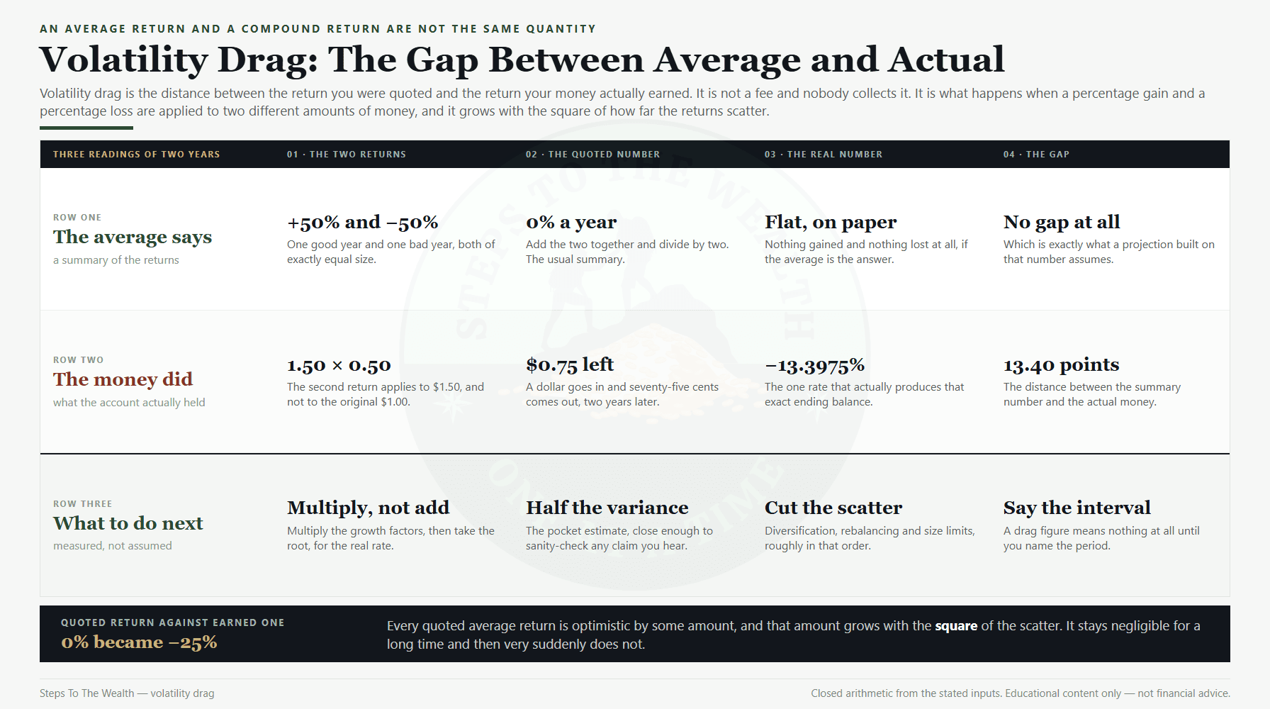
Somebody told you the market returns about 10% a year. You put 10% into a compounding calculator, watched the curve bend upward, and wrote down the number it landed on. That number is almost certainly too high — not because the 10% was a lie, but because an average return and a compound return are two different quantities, and only one of them is what ends up in the account.
The gap between them is volatility drag. It is not a fee, not a tax, and not something a broker is quietly taking from you. It is arithmetic. Multiply a sequence of returns together and the result is always smaller than the same returns added up and divided — unless every single one of them is identical. The more they scatter, the wider the gap gets, and it widens faster than the scatter does.
This article is the arithmetic, worked in full, with every number closed from the inputs on the page. No backtest, no forecast, nothing you cannot check on a calculator in about ninety seconds.
What volatility drag actually is
Two numbers can describe the same run of returns. The arithmetic average adds them up and divides by how many there were. The compound return asks a different question: what single steady rate, repeated every period, would have produced the exact ending balance you actually got?
Only the second one is real. It is the rate your money truly grew at. The first is a summary statistic that happens to be easy to compute, and it is the one that gets quoted, because it is bigger and because most people never learn there is a difference.
Volatility drag is the distance between the two. It appears for one reason: gains and losses are not symmetrical in their effect. A loss shrinks the base that the next gain has to work on, so a 10% recovery after a 10% fall does not get you back to level. That asymmetry is the same one at work in the arithmetic of recovery, seen from the other side.
Three things follow, and they are worth stating before any of the numbers arrive:
- The compound return is always less than or equal to the arithmetic average. There is no arrangement of returns where it comes out higher.
- They are equal in exactly one case: when every return in the run is the same number.
- The gap grows with the square of how much the returns scatter, which is why it stays trivial for a while and then stops being trivial rather suddenly.
Two returns that average zero and still lose a quarter
Start with the smallest example that shows the whole problem. Two years. The first returns +50%. The second returns −50%.
Add them and divide: the arithmetic average is 0% a year. Nothing gained, nothing lost, on paper.
Now run the money through it. A dollar becomes $1.50 at the end of year one. Then it falls by half: $1.50 × 0.50 = $0.75. You are down 25%, and the average return told you that you were flat.
The compound rate is the square root of 0.75, minus one: −13.3975% a year. That is the honest number. The 0% was not a rounding error or a bad estimate. It was the wrong statistic answering a question nobody asked.
The mechanism is visible in one line. The 50% gain is measured against $1.00. The 50% loss is measured against $1.50. The percentages match; the dollars they apply to do not. Whenever a sequence goes up and then down, the down applies to a bigger base — and whenever it goes down and then up, the up applies to a smaller one. Either order, same ending balance, same shortfall.
This is also why order does not matter here but matters enormously once you are adding or withdrawing money. Multiplication does not care about sequence. Cash flows do, and that is a separate problem with its own arithmetic, covered in sequence of returns risk.
Why the gap widens faster than the swing
Run the same two-year structure at different swing sizes and the shape of the problem becomes clear. Each row below has an arithmetic average of exactly 0%. The only thing that changes is how far the two returns sit from it.
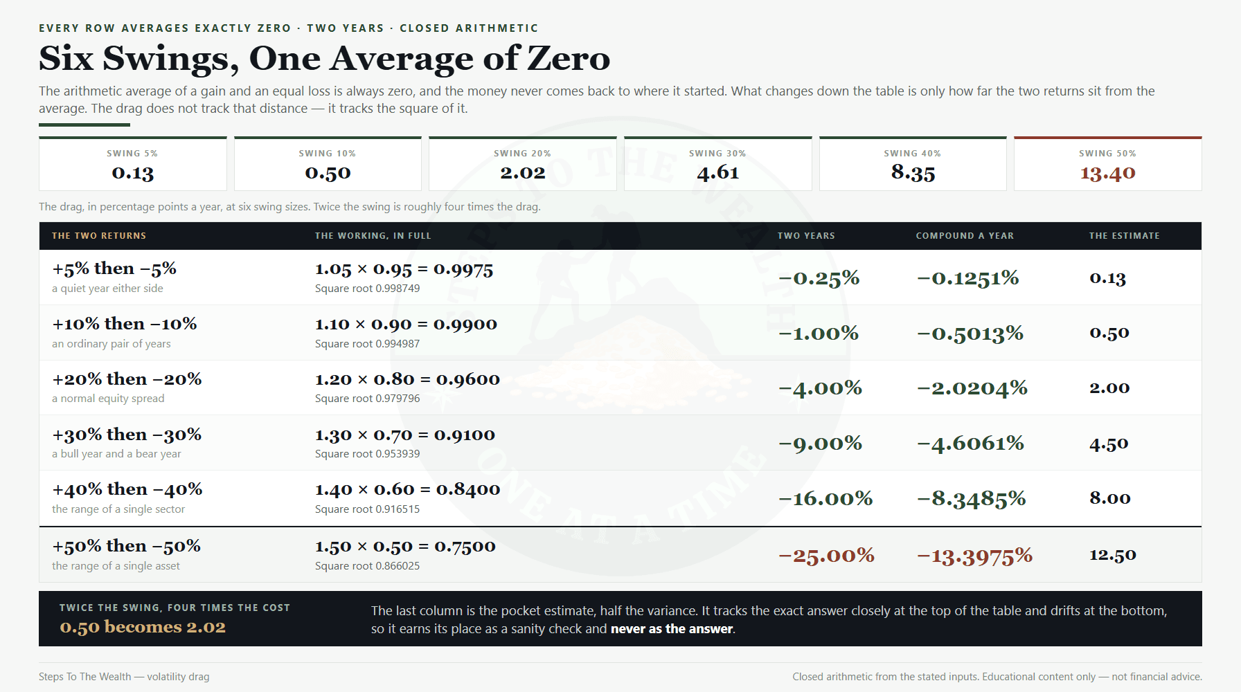
Read the last column against the second-to-last. At a ±5% swing the drag is 0.13 percentage points a year — genuinely ignorable. At ±20% it is 2.02 points. At ±50% it is 13.40 points, which is larger than the entire long-run return of most diversified portfolios.
Doubling the swing does not double the drag. Going from ±10% to ±20% takes the drag from 0.50 to 2.02 — roughly four times, for twice the movement. That is the squared relationship showing up in the table rather than in a formula, and it is the single most useful thing to carry out of this article. Small amounts of volatility cost almost nothing. Large amounts cost more than people expect, and the transition between those two states is not gradual.
Three portfolios, one average, three different endings
Zero-average examples make the mechanism obvious but feel artificial, so here is the same arithmetic with a return you would actually want. Three portfolios. Each one has an arithmetic average of exactly 8% a year over two years. Nothing else about them matches.
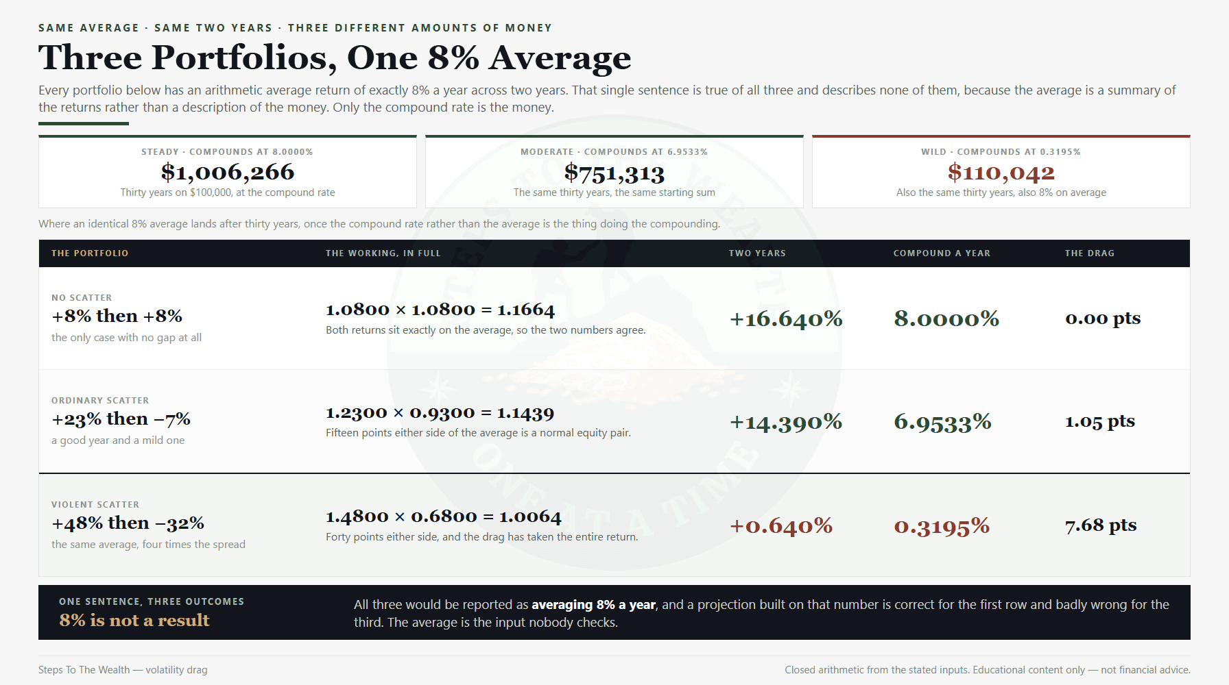
The steady portfolio earns 8% twice. It ends at 1.0800 × 1.0800 = 1.1664, up 16.640%, and its compound rate is 8.0000% — identical to its average, because its returns never scattered at all.
The moderate portfolio earns 23% then loses 7%. Same 8% average. It ends at 1.23 × 0.93 = 1.1439, up 14.390%, compounding at 6.9533%. The drag is 1.05 points a year.
The wild portfolio earns 48% then loses 32%. Still an 8% average. It ends at 1.48 × 0.68 = 1.0064 — up 0.640% across two years, compounding at 0.3195%. The drag is 7.68 points, and it has eaten essentially the entire return.
All three would be described by the same sentence: “it averaged 8% a year.” Across thirty years the first ends with 34% more capital than the second, and the third ends with about a ninth of the first. If you have ever wondered why comparing your portfolio to a benchmark is harder than it looks, this is a large part of the reason — the headline number is not describing what you think it is describing.
The estimate worth memorising
There is a pocket version of all of this. The compound return is approximately the arithmetic average minus half the variance:
compound ≈ average − (σ² ÷ 2)
Where σ is the standard deviation of the returns, expressed as a decimal. For a portfolio averaging 8% with a 15% standard deviation, that is 0.15² ÷ 2 = 0.01125, or about 1.13 percentage points of drag.
Check it against the moderate portfolio above. Its two returns sit 15 points either side of 8%, so σ is 0.15 and the estimate says 1.13 points. The exact answer, computed from the actual multiplication, was 1.05 points. Close, and slightly too pessimistic.
Now check it on the ±50% row from the earlier table. The estimate says 0.50² ÷ 2 = 12.50 points. The exact answer was 13.40. Close again, and this time too optimistic.
So the rule errs in both directions, depending on the average it is sitting on top of. Treat it as a sanity check, not an answer. When the number matters — when you are deciding something on it — multiply the actual returns together and take the root. The exact two-period identity is short enough to keep: with an average a and a deviation d, the compound rate is the square root of (1 + a)² − d², minus one.
What the same average does over ten years
Two periods keep the arithmetic checkable, but they understate the consequence, because drag is a rate and rates compound. Here is the same idea run over ten years, on $10,000, with an arithmetic average of exactly 10% a year in every column.
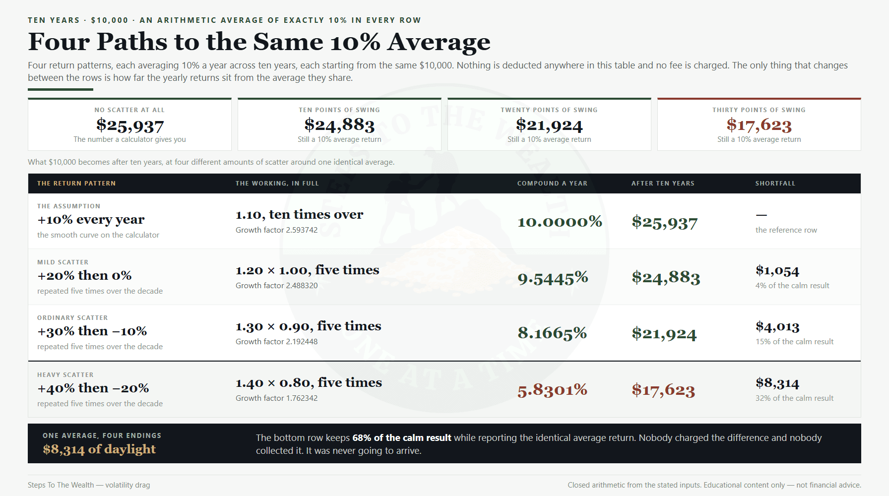
With no scatter at all, 10% a year for ten years turns $10,000 into $25,937. Alternate +20% and 0% — still a 10% average — and it becomes $24,883. Alternate +30% and −10% and it is $21,924. Alternate +40% and −20% and you finish with $17,623.
Same average return in all four columns. A $8,314 spread in the ending balance, which is 32% of the calm result. Nobody was charged anything, nobody made a bad decision, and no fee was deducted. The four columns simply had different amounts of scatter around an identical mean.
Stretch that to thirty years and the three portfolios from the previous section separate brutally. $100,000 compounding at 8.0000% reaches $1,006,266. At 6.9533% it reaches $751,313. At 0.3195% it reaches $110,042. One sentence described all three: “averaged 8% a year.”
Where the number you were quoted came from
None of this means published average returns are dishonest. Most of them are arithmetic averages because that is the conventional way to report a series, and the convention is fine as long as everyone knows which number they are holding.
The problem is what happens next. A 10% arithmetic average goes into a retirement projection as though it were a compound rate, and the projection comes out too high — not by a rounding error, but by whatever the drag happens to be for that portfolio, compounded across every remaining year.
Here is a realistic shape of it. Nine years at +12% and one year at −35%. The arithmetic average is 7.30% a year. The money grows by 80.25% in total, which is a compound rate of 6.0688%. The drag is 1.23 points, and one bad year in ten did all of it.
That is the honest version of a “good decade.” It is also why the phrase average annual return deserves a follow-up question every time it appears: averaged how? If the answer is “added up and divided,” you are holding the optimistic number. The distinction between measuring an asset and measuring your own money is worked through in full in XIRR vs CAGR.
Why the measurement interval changes the answer
There is a caveat that sits underneath every number in this article, and skipping it is how people end up arguing about drag figures that are both correct.
Volatility drag is not a property of an asset on its own. It is a property of an asset and the interval you measure it over. Take the +50% / −50% pair from earlier and make them two halves of a single year instead of two separate years. The money still ends at $0.75, so the annual return for that year is −25%.
Now look at what each observer sees. Someone with annual data has exactly one number, −25%, and one number cannot scatter, so they measure a drag of zero. Someone with semi-annual data sees a 0% average and a −13.3975% compound rate per half-year, and measures 13.40 points of drag. Neither of them is wrong, and neither of them is looking at a different portfolio.
The finer the interval, the more scatter you capture and the larger the drag you compute. This is why a fund’s daily volatility and its annual volatility tell different stories about the same year, and why the effect is at its most extreme in products that reset their exposure every day — a mechanism worth understanding separately, because it is a different animal from ordinary portfolio drag.
The practical rule is short. Use the same interval for the average and for the compound rate, use annual data unless you have a specific reason not to, and say which interval you used whenever you quote a drag number to anyone, yourself included.
What actually shrinks volatility drag
Because the drag scales with the square of the scatter, anything that genuinely lowers portfolio volatility pays back more than it appears to. Three things do, and it is worth being precise about how each one works.
Diversification across things that do not move together. Combining assets whose returns are not perfectly correlated produces a portfolio whose volatility is lower than the weighted average of the parts. That is the one structural reduction available without giving up expected return, and the mechanism is set out in how diversification reduces risk and in the regulator’s own primer on asset allocation. It also has limits, which show up precisely when you need them not to.
Rebalancing. Selling what has run and buying what has lagged pulls the portfolio back toward its target weights, which caps how far any one holding can drag the whole. The effect is real but modest, and it is not the free lunch it sometimes gets sold as — the trade-offs are laid out in rebalancing versus chasing.
Position sizing. The most direct lever. A high-volatility holding contributes drag in proportion to the square of its weight, so halving a position cuts its contribution to portfolio variance to roughly a quarter. This is the arithmetic underneath position sizing rules, and it is why a small allocation to something violent is a genuinely different decision from a large one, not just a smaller version of the same one.
The squared relationship is what makes position sizing the sharpest of the three. Cutting a holding’s weight from 20% to 10% does not halve its contribution to portfolio variance — it takes that contribution to a quarter, because the weight enters squared. A violent sleeve held at a small weight is close to harmless; the same sleeve at a large weight can dominate the portfolio’s entire drag figure on its own. That is a structural argument for size limits, and it holds whether or not you have any view on what the holding will do next.
What does not shrink it: predicting which years will be the bad ones. That is market timing wearing a mathematical costume, and the drag arithmetic gives you no edge in doing it.
What volatility drag is not
This concept gets misused in two opposite directions, and both are worth naming.
It is not a reason to avoid volatile assets. Drag reduces the return of a volatile holding; it does not automatically reduce it below a calm one. An asset with a 20% arithmetic average and 30% volatility compounds at roughly 15.5% — still far ahead of a steady 6%. The question is never “does this have drag,” because everything that moves has drag. The question is whether the expected return survives it, which is the same comparison run in the S&P 500 against Bitcoin.
It is not a hidden charge. Nothing is deducted. There is no counterparty on the other side of volatility drag collecting it. The money was never there — the arithmetic average simply described a quantity that was never going to arrive. Treating drag as a cost to be recovered leads directly to products that promise to “capture” it, and there is nothing to capture. Real deductions are a separate matter, and those are worth being furious about: see the hidden cost of investment fees.
It is not the same as sequence risk. Drag is about how far returns scatter and shows up even with no cash flows at all. Sequence risk is about what order they arrive in, and only exists when money is going in or coming out. A portfolio you never touch has drag and no sequence risk. Both are real, they are not the same thing, and confusing them produces bad conclusions in both directions.
It is not captured by a single risk number either. A volatility figure on a fund factsheet tells you the scatter but not what it costs you, and a risk-adjusted ratio folds them together in a way that hides the split — the limits of that are worked through in the Sharpe ratio explained.
How to measure your own
The measurement takes about ten minutes once a year, and it needs nothing but your own statements.
First, get your annual returns for each of the last several years. Second, add them and divide — that is your arithmetic average, and it is the number you have probably been quoting to yourself. Third, multiply the growth factors together instead: a +12% year is 1.12, a −8% year is 0.92. Take the result to the power of one over the number of years, subtract one, and that is your compound return.
The difference between the two is your volatility drag, in percentage points a year. If it is under half a point, the scatter in your portfolio is not costing you anything worth restructuring for. If it is over two points, the scatter is now a larger factor in your outcome than most of the decisions you spend time on.
Then do the thing that actually changes the answer: check what the same plan would have produced across a real drawdown rather than a smooth assumption. That is what the DCA Simulator exists for, and it reports the compound result rather than the average, which is the whole point. If you would rather see the framework applied week by week instead, the Sunday newsletter is where it runs.
One caution on the measurement itself. If you were contributing money throughout the period — and most working investors are — then a compound return computed on the asset is still not the return on your dollars. That is a third number again, and the doubling arithmetic is a quick way to sanity-check whichever one you end up with.
The takeaway
An average return and a compound return answer different questions, and the gap between them is volatility drag. It is not a fee and nobody is taking it. It is the price of the fact that a percentage gain and a percentage loss apply to different amounts of money.
The practical version fits in three lines. Every quoted average return is optimistic by some amount. That amount grows with the square of how much the returns scatter, so it stays negligible and then very suddenly is not. And the only way to know which side of that line your own portfolio sits on is to multiply the years together instead of adding them.
Run your own numbers. It takes ten minutes, and it is the rare measurement that changes what you do next.
Educational content only — not financial advice.